General Utilities

CartoBoost includes numerical utilities that can be used without building a CartoBoostRegressor or a forecasting ForecastFrame. Use these when you have a plain Python sequence, a small spatial interpolation problem, or an intermittent-demand sequence and want a direct result.

These functions are useful for scientific checks and ablations: they let you compare a full estimator or forecasting wrapper against the same underlying method on a simple zone sequence, route panel, or coordinate interpolation problem.

import cartoboost as cb

Sequence Reference Utilities

Use cartoboost.forecasting.sequence when a row sequence has a known target prefix, a target-missing prediction suffix, and an external reference axis such as a canonical demand profile. The utilities validate the prefix/suffix boundary and reject target leakage in prediction rows.

from cartoboost.forecasting import (
    ReferenceSignal,
    SequenceRow,
    SequenceSeries,
    forward_ekf,
    reference_path_viterbi,
)

series = SequenceSeries(
    "location_142",
    [
        SequenceRow("hour_00", 0.0, 0.0),
        SequenceRow("hour_01", 1.0, 1.0),
        SequenceRow("hour_02", 2.0, None),
    ],
)
reference = ReferenceSignal(axis=[0.0, 1.0, 2.0], signal=[0.0, 1.0, 2.0])

filtered = forward_ekf(series, reference)
path = reference_path_viterbi(series, reference)

Available entry points:

Entry point	Purpose
validate_sequence_frame	Validates finite ordered positions, nonempty known prefixes, nonempty prediction suffixes, monotonic deduplicated reference axes, and no target leakage into prediction rows.
forward_ekf, ukf_reference, rts_smoother	State-space continuation over a reference signal with configurable process and observation noise plus optional auxiliary rate observations.
missing_target_continuation	Returns only prediction-suffix continuation rows after fitting from the known prefix.
reference_path_viterbi	Discrete robust-emission Viterbi path over a reference axis.
reference_path_posterior_mean	Forward-backward posterior mean path bounded by the reference axis.
sequence_blend	Fixed, validation-derived, or constrained nonnegative candidate blending over aligned sequence row IDs.
generate_group_oof_candidate_rows, validate_oof_meta_training, per_group_error_summary	Leakage-safe group-level OOF candidate row generation, meta-training checks, and per-group RMSE/MAE summaries.

Local-Level Kalman

Use local-level Kalman filtering when the signal is a noisy measurement of a slowly moving level and there is no explicit trend term.

Example: a location counter reads a stable hourly demand level with small noise, and you want a smoothed level plus a short flat forecast.

import cartoboost as cb

readings = [99.0, 101.0, 100.0, 102.0, 101.0, 103.0]

state = cb.local_level_kalman_filter(
    readings,
    level_process_variance=0.05,
    observation_variance=1.0,
    horizon=3,
)

print(state["final_state"]["level"])
print(state["forecast"])

For just the forecast means:

forecast = cb.local_level_kalman_forecast(
    readings,
    horizon=3,
    level_process_variance=0.05,
    observation_variance=1.0,
)

Parameters:

Parameter	Meaning
level_process_variance	How much the latent level is allowed to move between observations. Larger values adapt faster.
observation_variance	Measurement noise. Larger values smooth the observations more strongly.
horizon	Number of future means to emit from the filtered final state.

Return shape:

• local_level_kalman_filter(...) returns a dictionary with per-step estimates, final level state, fixed-interval smoothed_states, optional forecast, optional forecast_distribution, and diagnostics.
• Each estimate includes the prior level, filtered level, variances, innovation, fitted value, residual, standardized innovation, Kalman gain, and per-step Gaussian log likelihood.
• forecast_distribution rows include step, mean, observation variance, and normal-approximation lower/upper bounds. Use interval_z to control the interval width.
• diagnostics includes log likelihood, AIC, BIC, MSE, RMSE, MAE, and standardized-innovation summaries.
• local_level_kalman_forecast(...) returns list[float].

Visualization example:

import matplotlib.pyplot as plt
import cartoboost as cb

readings = [184.0, 187.0, 183.0, 186.0, 185.0, 188.0, 186.0]
state = cb.local_level_kalman_filter(readings, horizon=3)

steps = list(range(len(readings)))
smoothed_steps = [row["step"] for row in state["smoothed_states"]]
smoothed = [row["level"] for row in state["smoothed_states"]]
future_steps = [steps[-1] + row["step"] for row in state["forecast_distribution"]]
future_mean = [row["mean"] for row in state["forecast_distribution"]]
future_lower = [row["lower"] for row in state["forecast_distribution"]]
future_upper = [row["upper"] for row in state["forecast_distribution"]]

plt.plot(steps, readings, marker="o", label="observed zone pickups")
plt.plot(smoothed_steps, smoothed, label="smoothed level")
plt.plot(future_steps, future_mean, marker="o", label="forecast")
plt.fill_between(future_steps, future_lower, future_upper, alpha=0.18)
plt.legend()
plt.savefig("target/examples/local_level_kalman_utility.png", dpi=160)

Local-Linear-Trend Kalman

Use local-linear Kalman filtering when the series has a level and a slope. This matches load, traffic, or pickup counts that drift over time.

Example: daily pickup demand is increasing by about two trips per day, with noise.

import cartoboost as cb

pickups = [40.0, 42.0, 45.0, 47.0, 50.0, 51.0, 54.0]

state = cb.kalman_filter(
    pickups,
    level_process_variance=0.05,
    trend_process_variance=0.005,
    observation_variance=0.5,
    horizon=4,
)

print(state["final_state"]["level"], state["final_state"]["trend"])
print(state["forecast"])

For just the forecast means:

forecast = cb.local_linear_trend_kalman_forecast(
    pickups,
    horizon=4,
    level_process_variance=0.05,
    trend_process_variance=0.005,
    observation_variance=0.5,
)

Parameters:

Parameter	Meaning
level_process_variance	Process noise for the latent level.
trend_process_variance	Process noise for the latent trend/slope.
observation_variance	Measurement noise in the observed values.
horizon	Number of future means to emit from the final level/trend state.
interval_z	Normal critical value used for forecast_distribution bounds when horizon > 0.

Return shape:

• kalman_filter(...) returns final level/trend state, final covariance, fixed-interval smoothed_states, per-step estimates, optional point forecast, optional forecast_distribution, and diagnostics.
• Each local-linear estimate includes prior and filtered state values, covariance matrices, fitted value, residual, standardized innovation, innovation variance, level/trend gains, and per-step Gaussian log likelihood.
• diagnostics includes log likelihood, AIC, BIC, MSE, RMSE, MAE, and standardized-innovation summaries.

Visualization example:

import matplotlib.pyplot as plt
import cartoboost as cb

pickups = [40.0, 42.0, 45.0, 47.0, 50.0, 51.0, 54.0]
state = cb.kalman_filter(pickups, horizon=4)

steps = list(range(len(pickups)))
estimate_steps = [row["step"] for row in state["estimates"]]
filtered = [row["level"] for row in state["estimates"]]
fitted = [row["fitted"] for row in state["estimates"]]
future_steps = [steps[-1] + row["step"] for row in state["forecast_distribution"]]
future_mean = [row["mean"] for row in state["forecast_distribution"]]
future_lower = [row["lower"] for row in state["forecast_distribution"]]
future_upper = [row["upper"] for row in state["forecast_distribution"]]

plt.plot(steps, pickups, marker="o", label="observed pickup count")
plt.plot(estimate_steps, fitted, linestyle="--", label="one-step fitted")
plt.plot(estimate_steps, filtered, label="filtered level")
plt.plot(future_steps, future_mean, marker="o", label="forecast")
plt.fill_between(future_steps, future_lower, future_upper, alpha=0.18)
plt.legend()
plt.savefig("target/examples/local_linear_kalman_utility.png", dpi=160)

Forecasting wrapper:

Use KalmanForecaster when you want the same local-linear model behind the forecasting API.

from cartoboost.forecasting import KalmanForecaster

model = KalmanForecaster(
    level_process_variance=0.05,
    trend_process_variance=0.005,
    observation_variance=0.5,
)
model.fit([40.0, 42.0, 45.0, 47.0, 50.0, 51.0, 54.0])
result = model.predict(4)

print(result.predictions())

Panel input is also supported:

model.fit(
    {
        "location_142": [40.0, 42.0, 45.0, 47.0],
        "location_236": [70.0, 69.0, 68.0, 66.0],
    }
)

Ordinary Kriging

Use ordinary kriging when you have observed values at known coordinates and want spatial interpolation at new coordinates. The utility is independent of forecasting. The forecasting wrapper uses the latest observed value for each series and interpolates across panel coordinates.

Example: three locations have observed demand pressure, and you want the estimated pressure at a nearby centroid.

import cartoboost as cb

observations = [
    (0.0, 0.0, 10.0),  # x, y, value
    (1.0, 0.0, 20.0),
    (0.0, 1.0, 14.0),
]
targets = [
    (0.25, 0.25),
    (0.75, 0.10),
]

predictions = cb.ordinary_kriging_predict(
    observations,
    targets,
    range=1.5,
    nugget=1.0e-6,
    variogram_model="spherical",
    detailed=True,
)

for row in predictions:
    print(row["x"], row["y"], row["mean"], row["variance"], row["neighbor_indices"])

Parameters:

Parameter	Meaning
observations	Sequence of (x, y, value) triples.
targets	Sequence of (x, y) coordinates to interpolate.
range	Distance scale for bounded semivariograms. For linear, it is the denominator of the slope sill / range.
nugget	Non-negative origin discontinuity representing an uncorrelated or measurement-scale component.
sill	Structural semivariance contribution for bounded models; for linear, the contribution at distance range.
variogram_model	exponential, gaussian, spherical, or linear.
drift	ordinary for constant mean or linear for universal kriging with x/y drift.
anisotropy_angle_degrees, anisotropy_scaling	Rotate and stretch the spatial distance metric.
max_neighbors, min_neighbors, max_distance	Optional target-local neighbor selection. All-neighbor predictions cache the kriging system once for faster many-target scoring.
detailed	When true, include kriging variance and selected neighbor indices.

For positive distance d, the exponential and Gaussian models use nugget + sill * (1 - exp(-d / range)) and nugget + sill * (1 - exp(-(d / range)^2)). The spherical model rises as nugget + sill * (1.5r - 0.5r^3) for r = d / range < 1 and then stays at nugget + sill. The linear model uses the unbounded semivariogram nugget + (sill / range) * d; its range is a scale parameter, not a cutoff. The kriging system itself uses a zero diagonal.

Return shape:

• ordinary_kriging_predict(...) returns a list of dictionaries: {"x": ..., "y": ..., "mean": ..., "weights": [...]}.
• With detailed=True, each row also includes variance and neighbor_indices.
• ordinary_kriging_leave_one_out(...) returns the detailed row shape for each held-out observation and is intended for spatial residual diagnostics.
• empirical_variogram(...) returns binned semivariances with lag boundaries, mean lag distance, and pair counts.
• fit_ordinary_kriging_variogram(...) runs weighted least-squares selection over variogram, range, nugget, and sill candidates and returns the selected config plus the empirical bins and objective value.
• ordinary_kriging_leave_one_out_diagnostics(...) returns held-out predictions plus residual metrics such as bias, MAE, RMSE, standardized RMSE, 95% interval coverage, and average kriging variance.

Visual example walkthrough:

• Full example script: examples/forecasting/kriging_example_visualization.py
• Generated surface:
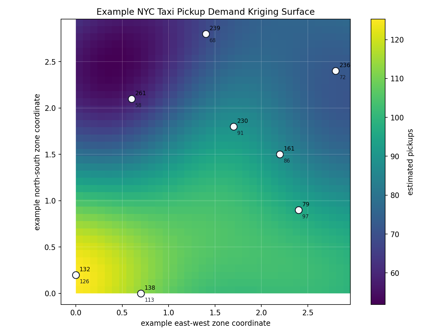
• Generated variogram:
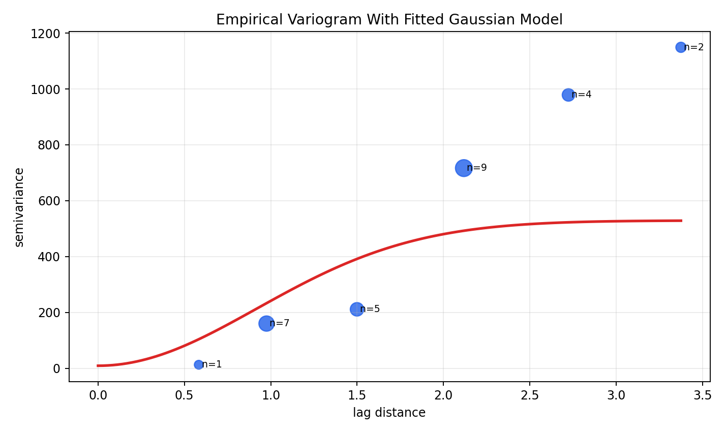
• Generated leave-one-out diagnostics:

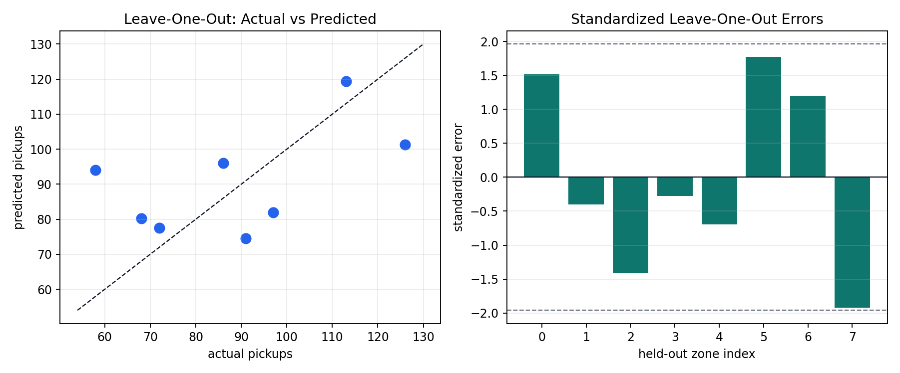
Forecasting wrapper:

Use KrigingForecaster when the data is a panel of series and each series has a fixed coordinate. The wrapper forecasts each series by kriging the latest known panel values at that series coordinate.

from cartoboost.forecasting import KrigingForecaster

coordinates = {
    "location_142": (0.0, 0.0),
    "location_236": (1.0, 0.0),
    "location_239": (0.0, 1.0),
}

model = KrigingForecaster(coordinates=coordinates, range=1.5, nugget=1.0e-6)
model.fit(
    {
        "location_142": [10.0, 12.0],
        "location_236": [20.0, 21.0],
        "location_239": [14.0, 15.0],
    }
)
result = model.predict(1)

print(result.predictions())

Coordinates can also be passed as triples:

KrigingForecaster(
    coordinates=[
        ("location_142", 0.0, 0.0),
        ("location_236", 1.0, 0.0),
    ],
)

Intermittent Demand

Use Croston-family utilities when demand is non-negative and contains many zeros. They are useful for sparse demand requests, low-volume parts, or rare lane/customer activity.

Example: a low-volume lane has several zero-demand days and occasional orders.

import cartoboost as cb

demand = [0.0, 0.0, 4.0, 0.0, 0.0, 2.0, 0.0, 5.0, 0.0]

croston = cb.croston_forecast(demand, horizon=5, alpha=0.2)
sba = cb.sba_forecast(demand, horizon=5, alpha=0.2)
tsb = cb.tsb_forecast(demand, horizon=5, alpha=0.2, beta=0.1)

print(croston)
print(sba)
print(tsb)

Method guide:

Method	Entry point	Use when
Croston	croston_forecast or intermittent_demand_forecast(method="croston")	You need a simple baseline for sparse non-zero events.
SBA	sba_forecast or intermittent_demand_forecast(method="sba")	You want Croston with a standard bias adjustment.
TSB	tsb_forecast or intermittent_demand_forecast(method="tsb")	You want separate smoothing for event probability and non-zero demand size.

Inputs must be finite and non-negative. The output is a list[float] of length horizon.

Single-Series Forecast Utilities

The same local models used by forecasting wrappers can be called on plain numeric sequences:

import cartoboost as cb

values = [20.0, 21.0, 19.0, 22.0, 23.0, 24.0, 26.0]

print(cb.naive_forecast(values, horizon=3))
print(cb.seasonal_naive_forecast(values, horizon=3, season_length=7))
print(cb.theta_forecast(values, horizon=3))
print(cb.optimized_theta_forecast(values, horizon=3))
print(cb.ets_forecast(values, horizon=3, alpha=0.5, beta=0.1))
print(cb.arima_forecast(values, horizon=3, p=1, d=1, q=0))
print(cb.auto_arima_forecast(values, horizon=3, max_p=2, max_d=1, max_q=1))

Use series_forecast when the model name is dynamic:

forecast = cb.series_forecast(
    "local_linear_trend_kalman",
    values,
    horizon=3,
    level_process_variance=0.05,
    trend_process_variance=0.005,
    observation_variance=1.0,
)

Choosing A Utility

Problem shape	Default utility
Noisy stable level	local_level_kalman_filter
Noisy level plus slope	kalman_filter or local_linear_trend_kalman_forecast
Spatial interpolation from coordinate samples	ordinary_kriging_predict
Sparse non-negative demand	sba_forecast or tsb_forecast
Quick local time-series baseline	series_forecast or the named forecast helpers

Geotemporal Forecast Utilities

CartoBoost also exposes reusable utilities for geotemporal model diagnostics and uncertainty control. These are lower-level primitives for model authors and benchmark harnesses when a workflow needs calibrated intervals, residual-state correction, regime detection, or probability calibration.

Primitive family	Use
QuantileLoss, HuberQuantileLoss, CompositeQuantileLoss, QuantileRegressorSet	Fit and score calibrated p10/p25/p50/p75/p90-style quantile bundles with non-crossing repair, pinball loss, interval width, coverage, and crossing-rate diagnostics.
ConformalCalibrator	Serializable split-conformal residual calibration for interval coverage.
KalmanResidualCorrector, StateFilter, StateCorrectedBooster	Add leakage-safe residual-state corrections after structural booster predictions, using predict-before-update ordering and optional origin, destination, corridor, segment, entity-family, target-family, and time-bucket state keys.
CUSUM, PageHinkley, EwmaVolatility, rolling median residuals, rolling MAD residuals	Detect mean shifts or volatility changes and feed regime-aware interval policies.
RegimeIntervalPolicy	Widen intervals, raise process variance, or lower confidence during detected shifts.
SigmoidCalibrator, TemperatureCalibrator, IsotonicCalibrator	Calibrate binary event probabilities with bounded outputs, Brier score, log loss, ECE, calibration buckets, and reliability-curve data.

Supported event helpers include success within a threshold, event within a horizon, failure risk, and escalation risk. Use them when the forecasting question needs a calibrated probability such as "pickup demand exceeds this threshold within the next six hours" rather than only a point forecast.