Kriging

KrigingForecaster is an ordinary-kriging panel forecaster. It borrows signal across series using explicit coordinates keyed by series id.

Kriging is most useful when the thing being forecast has spatial structure: nearby locations should be related to nearby locations, and route midpoint aggregates can share signal with nearby corridors. CartoBoost exposes both the panel forecaster and lower-level utilities for one-off interpolation, variogram fitting, and residual diagnostics.

Interactive Example

Kriging coordinate-panel forecast

Runs kriging against a bundled multi-location demand panel sample.

Ready to run in this page.

When To Use

Use kriging when nearby locations or route midpoints should have related future values. Every series id in the training panel should have a coordinate.

Good fits usually have these properties:

• stable series ids such as location ids or route ids,
• a coordinate for every training series id,
• enough neighboring zones to estimate spatial correlation,
• validation folds that preserve time order,
• a reason to expect geography to explain residual variation after calendar and lag features.

Avoid kriging as the only model when the signal is mostly temporal, such as a single-series rush-hour pattern. In that case, compare against seasonal naive, Kalman, ARIMA, or a lag model with hour/day features. Kriging is strongest when spatial borrowing adds information that a per-series temporal model cannot see.

Scientific Role

Kriging is a spatial covariance model. It asks whether differences between series are related to coordinate distance after the chosen temporal summary has been formed. A scientist should choose it when geography is part of the mechanism being tested, not merely because locations have coordinates.

For panel demand, a defensible kriging claim is: nearby locations or route midpoints have correlated residual demand, and the variogram plus neighbor rules make that borrowing explicit. The model is weaker as a pure time-series forecaster because it does not learn hour-of-day dynamics by itself.

Assumptions And Failure Modes

Kriging assumes the coordinate system, variogram, and neighbor controls describe how spatial similarity decays. It also assumes that every series id has a stable, meaningful coordinate and that missing coordinates are input errors, not values to invent.

Failure modes include smooth surfaces that hide sharp airport or venue effects, edge predictions unsupported by nearby observations, variograms with no clear distance pattern, and zones whose demand is driven more by calendar or route mix than by geometric proximity. Use leave-one-out diagnostics and time-ordered validation before treating a spatial surface as forecast evidence.

Python Example

from cartoboost.forecasting import KrigingForecaster

coordinates = {
    "132": (-73.7781, 40.6413),  # location 132
    "161": (-73.9776, 40.7580),  # Midtown
    "236": (-73.9577, 40.7808),  # Upper East Side
}

series = {
    "132": [120, 118, 125, 140, 155, 160],
    "161": [80, 84, 91, 105, 118, 121],
    "236": [62, 65, 70, 78, 85, 88],
}

model = KrigingForecaster(
    coordinates=coordinates,
    range=2.0,
    nugget=1.0e-6,
    variogram_model="spherical",
    max_neighbors=32,
    min_neighbors=3,
)
model.fit(series)
forecast = model.predict(3)

for row in forecast.predictions():
    print(row)

This panel form forecasts every training zone at the requested horizon. The model uses the latest value from each series and predicts each target zone from the spatial dependence implied by the coordinates and variogram settings.

ForecastFrame Example

from cartoboost.forecasting import ForecastFrame, KrigingForecaster

frame = ForecastFrame.from_pandas(
    hourly_zone_demand,
    timestamp_col="pickup_hour",
    target_col="demand",
    series_id_col="series_id",
    freq="h",
)

zone_centroids = {
    "132": (-73.7781, 40.6413),
    "161": (-73.9776, 40.7580),
    "236": (-73.9577, 40.7808),
}

model = KrigingForecaster(
    coordinates=zone_centroids,
    range=2.0,
    nugget=1e-6,
    sill=1.0,
    variogram_model="exponential",
    drift="ordinary",
)
model.fit(frame)
forecast = model.predict(6)

The frame example is the usual production shape: aggregate observations to hourly counts, keep the stable series key, and pass a centroid table whose keys match those ids after string conversion.

Utility Workflow

Use the lower-level utilities before locking a KrigingForecaster configuration. They let you inspect the spatial surface and residual behavior at one timestamp or validation fold.

import cartoboost as cb

observations = [
    (-73.7781, 40.6413, 126.0),  # location 132
    (-73.8628, 40.7684, 113.0),  # location 138
    (-73.9776, 40.7580, 86.0),   # location 161
    (-73.9577, 40.7808, 72.0),   # location 236
]

fit = cb.fit_ordinary_kriging_variogram(
    observations,
    variogram_models=["exponential", "spherical", "gaussian"],
    range_candidates=[0.5, 1.0, 1.5, 2.0, 3.0],
    nugget_candidates=[0.0, 2.0, 5.0],
    sill_candidates=[50.0, 150.0, 300.0],
    bin_count=4,
)

targets = [
    (-73.90, 40.72),  # route midpoint or unobserved zone coordinate
    (-73.98, 40.75),
]
predictions = cb.ordinary_kriging_predict(
    observations,
    targets,
    detailed=True,
    **fit["config"],
)

print(fit["config"])
print(predictions[0]["mean"], predictions[0]["variance"])

Use detailed=True when a dashboard or QA notebook needs kriging variance, weights, and selected neighbor indices. The same fitted config can be copied to KrigingForecaster for repeated panel forecasting.

Practical Workflow

1. Aggregate the data to the grain you plan to forecast, for example hourly counts by series id.
2. Join or build a centroid table keyed by the same ids. For route-level models, use route midpoint coordinates or a carefully chosen corridor coordinate.
3. Pick one training timestamp or rolling fold and create (x, y, value) observations from the latest known value for each zone.
4. Fit a variogram candidate grid with fit_ordinary_kriging_variogram.
5. Plot the interpolation surface to check whether the surface respects known high-demand zones and spatial corridors.
6. Plot the empirical variogram to see whether semivariance generally increases with distance before flattening near the sill.
7. Run leave-one-out diagnostics. If held-out zones have large standardized errors, add temporal features, adjust neighbor limits, or treat the zone as a special case before using the fitted config in a forecaster.

Example Walkthrough

The runnable example script below creates eight locations with fixed coordinates, fits a variogram by weighted least squares, interpolates a dense grid, and runs leave-one-out diagnostics. The data is synthetic and intentionally small so the geometry and residual behavior are easy to inspect.

uv run python examples/forecasting/kriging_example_visualization.py \
  --output-dir docs/assets/kriging_examples

The fitted example configuration is recorded in docs/assets/kriging_examples/kriging_example_summary.json. For the committed run, the selected example variogram is Gaussian with range 1.3, nugget 9.0, and sill 520.0.

The script is deterministic and does not download data. It is designed as a documentation and smoke-test example for the Python kriging utilities, not as a public benchmark claim.

Interpolation Surface

The surface plot shows how observed pickup demand at named zones is interpolated over an example city coordinate plane. The white points are observed zones, the large numbers are example pickup counts, and the background is the kriging mean.

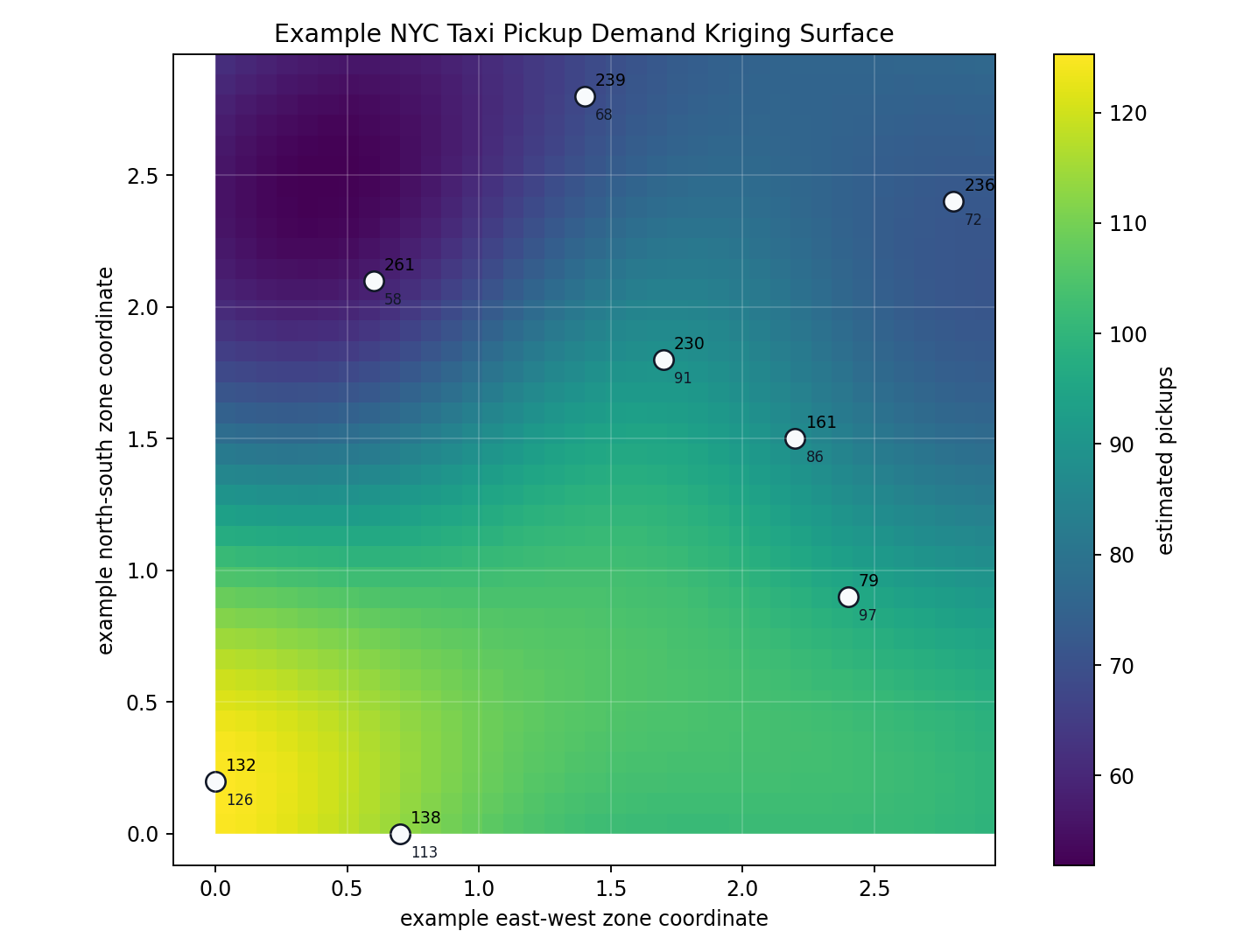
Interpret the surface as a spatial sanity check:

Pattern	Meaning	Typical next step
Smooth high-demand area around airport zones.	Nearby zones are borrowing signal as intended.	Validate against time-ordered folds before relying on the surface.
Sharp peaks around single observations.	Nugget or range may be too small, or the zone may be under-neighbored.	Increase range, increase min_neighbors, or compare a smoother variogram candidate.
Flat surface despite different observed values.	Sill may be too low or range too high.	Expand candidate grids and inspect leave-one-out error.
Edge predictions look implausible.	The target is outside well-supported observed geometry.	Avoid extrapolation claims or require nearby observed zones with max_distance.

Empirical Variogram

The variogram plot bins pairwise zone distances and semivariances. Bubble size tracks pair count, and the red line is the fitted theoretical model used by the interpolator.

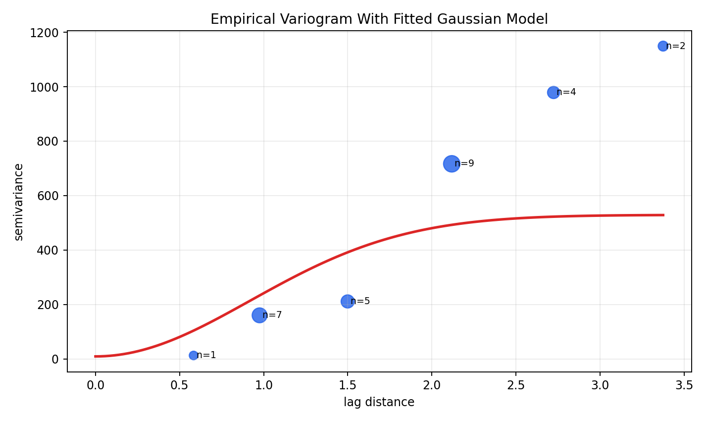
Use the variogram to decide whether the fitted spatial covariance is plausible:

Visual pattern	Meaning	Typical next step
Semivariance rises with distance then levels off.	Spatial covariance is visible at short lags.	Use the fitted config in rolling validation.
First bin has high semivariance.	Adjacent zones differ sharply.	Raise nugget, add route/calendar features, or segment airport/Midtown behavior.
No clear distance pattern.	Geography alone is weak for this target.	Prefer a temporal or lag model and use kriging only as a residual feature.
Sparse far-distance bins dominate the fit.	Pair counts are uneven.	Use weighted fitting and inspect bubble sizes before changing the candidate grid.

Leave-One-Out Diagnostics

The leave-one-out plot checks whether each observed pickup zone can be predicted from the remaining zones. The right panel standardizes residuals by kriging variance so unusually large spatial errors are visible.

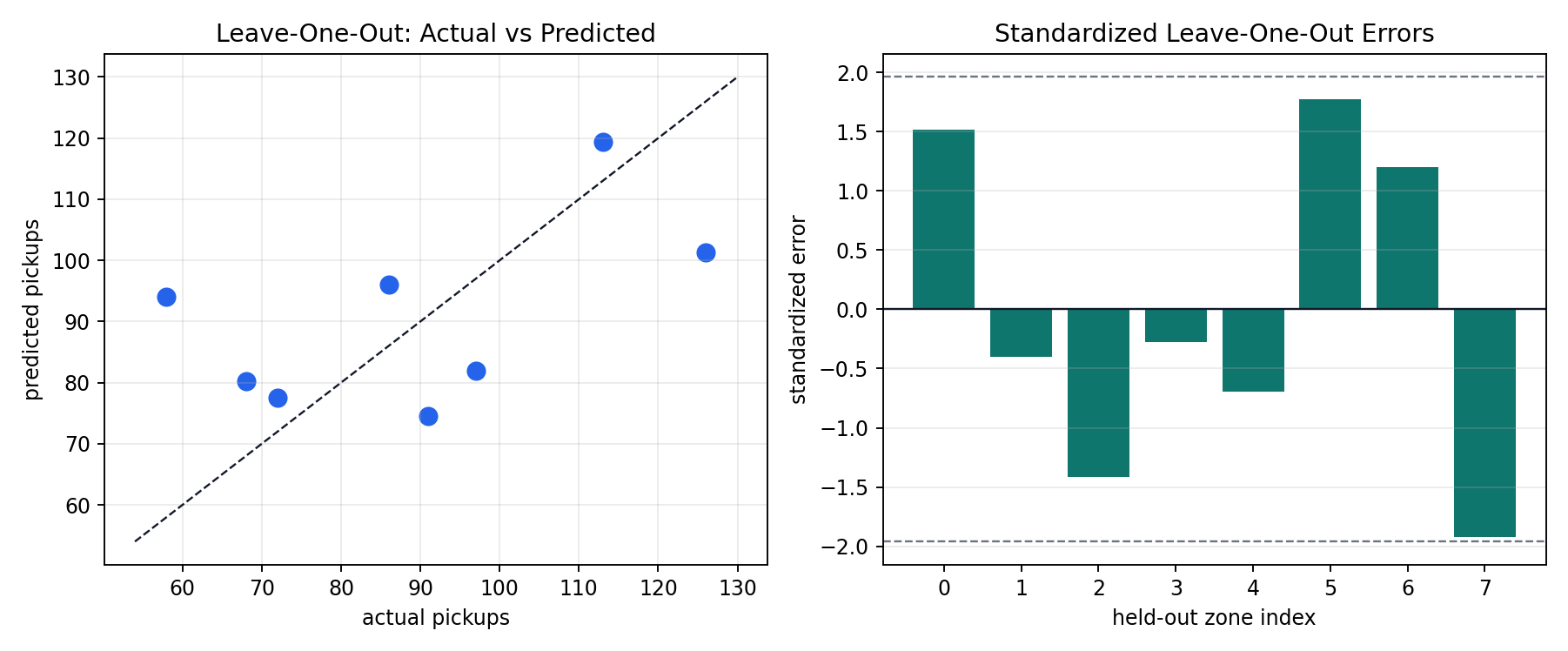
Use leave-one-out diagnostics to find zones that do not behave like their neighbors:

Diagnostic	Meaning	Typical next step
Actual-vs-predicted points follow the diagonal.	Spatial interpolation explains the held-out zones.	Move to rolling-origin validation.
One zone is far from the diagonal.	That zone has demand drivers not captured by coordinate distance.	Add calendar/airport flags, split route families, or cap its influence.
Standardized errors mostly stay within +/-1.96.	Kriging variance is roughly consistent with residual size.	Keep the interval configuration for validation.
Standardized errors are large but raw errors are modest.	Variance is too optimistic.	Increase nugget or sill candidate values.

The JSON summary written by the example records RMSE, MAE, mean error, average kriging variance, 95% interval coverage, and standardized residual summaries so that regenerated images can be compared with the committed documentation assets.

Parameters

Parameter	Notes
coordinates	Mapping from series id to (x, y) or rows of (series_id, x, y).
range	Distance scale for bounded variograms. For the linear model it sets the slope denominator.
nugget	Non-negative origin discontinuity representing an uncorrelated or measurement-scale component.
sill	Structural semivariance contribution for bounded models; for the linear model it is the contribution reached at range.
variogram_model	exponential, gaussian, spherical, or linear.
drift	ordinary for constant mean or linear for universal kriging with x/y drift.
anisotropy_angle_degrees, anisotropy_scaling	Rotate and stretch the spatial distance metric for directional taxi corridors.
max_neighbors, min_neighbors, max_distance	Optional local neighbor controls. When no local neighbor controls are set, the forecaster caches the fixed kriging system and reuses it across targets.

For positive separation distance d, the implemented semivariograms are:

Model	Semivariogram gamma(d)
exponential	nugget + sill * (1 - exp(-d / range))
gaussian	nugget + sill * (1 - exp(-(d / range)^2))
spherical	nugget + sill * (1.5r - 0.5r^3) for r = d / range < 1, then nugget + sill
linear	nugget + (sill / range) * d

The linear semivariogram is unbounded: range and sill determine its slope, not a plateau or cutoff. CartoBoost uses a zero diagonal in the kriging system; the nugget applies between distinct or target/observation locations.

Choosing Settings

Start with fitted utility parameters and then validate the forecaster. Do not tune the variogram only by making the surface look attractive.

Setting	Lower values	Higher values
range	Nearby zones dominate for bounded models; linear semivariance has a steeper slope for fixed sill.	Distant zones borrow more strongly for bounded models; linear semivariance has a shallower slope for fixed sill.
nugget	The model assigns less discontinuity to distinct or near-colocated observations.	The model allows a larger uncorrelated component.
sill	Bounded semivariograms have a lower structural plateau; the linear model has a shallower slope for fixed range.	Bounded semivariograms have a higher structural plateau; the linear model has a steeper slope for fixed range.
max_neighbors	Faster local prediction and less distant borrowing.	More stable global borrowing, but more compute and possible over-smoothing.
max_distance	Prevents extrapolation from far-away zones.	Allows broad citywide borrowing when local coverage is sparse.

drift="linear" can help when demand has a broad east-west or north-south gradient, but it should be validated against drift="ordinary" because a linear trend can absorb what should be local zone behavior. Use anisotropy when a taxi corridor has directional structure, such as a river crossing or airport access pattern where distance in one direction should count differently.

Diagnostics

For one-off coordinate interpolation, cartoboost.utilities.ordinary_kriging_predict(..., detailed=True) returns kriging variance and selected neighbor indices alongside the mean and weights. Use cartoboost.utilities.empirical_variogram(...) to inspect binned semivariances, cartoboost.utilities.fit_ordinary_kriging_variogram(...) to choose a range/nugget/sill/variogram model by weighted least squares, and cartoboost.utilities.ordinary_kriging_leave_one_out_diagnostics(...) to inspect leave-one-out bias, MAE, RMSE, standardized residuals, interval coverage, and average kriging variance before using the configuration in a panel forecaster.

Diagnostic rows are intended to be mechanical and scriptable. A focused QA check can hard-fail on finite metrics before writing benchmark or documentation claims:

diagnostics = cb.ordinary_kriging_leave_one_out_diagnostics(
    observations,
    **fit["config"],
)

metrics = diagnostics["diagnostics"]
assert metrics["observation_count"] == len(observations)
assert metrics["rmse"] >= 0.0
assert metrics["interval_coverage_95"] >= 0.0

Data Requirements

Kriging is panel-oriented. Use stable series ids such as location ids or route ids. Coordinate keys must match the string form of the series ids used by the forecasting frame or panel dictionary.

Coordinates can be projected coordinates, normalized city-plane coordinates, or longitude/latitude pairs for compact areas where the distance approximation is acceptable for the claim being made. For citywide benchmark claims, use a consistent coordinate system and keep the centroid source fixed across reruns. Do not silently invent coordinates for missing zones; fail the pipeline and fix the input table.

Validation

Kriging uses spatial proximity, not future observations. Validate with rolling-origin folds and consider a spatial holdout if the claim is about generalizing to unseen zones.

For forecasting claims, report RMSE, MAE, R2 when relevant, training time, prediction time, sample size, split boundaries, and the exact variogram and neighbor settings. Compare against serious temporal baselines on the same train/test split. If the kriging model is only used as a residual smoother or an interpolation utility, state that narrower role explicitly.

Limitations

• Quality depends on meaningful coordinates, distance units, and variogram assumptions.
• Nearby observations are not independent evidence under random row splits.
• Large panels may require neighbor limits or scalable GP alternatives.
• Spatial interpolation does not replace temporal baselines for forecasting claims.